Collect
SportsData.io salary and stat records are parsed into SQLite tables for more than 340 NBA players. The app keeps salary, biographical data, and box-score production in one combined table so predictions can be made with a fast local lookup.
Model notes
The app uses supervised machine learning to estimate a player's salary from production data, then compares that model price against the real contract number.
SportsData.io salary and stat records are parsed into SQLite tables for more than 340 NBA players. The app keeps salary, biographical data, and box-score production in one combined table so predictions can be made with a fast local lookup.
More than 50 statistics were screened against salary using Pearson correlation. The final model keeps 28 inputs across experience, total production, usage, PER, and per-game versions of high-signal stats like points, assists, rebounds, free throws, and turnovers.
Each feature is z-score normalized before training and prediction. That puts very different stat ranges on comparable scales, so total minutes or points do not automatically overpower smaller-scale inputs like usage rate or PER.
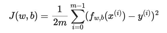
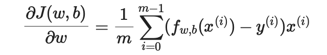
Linear regression is trained with gradient descent for 100,000 iterations using mean squared error as the cost function. The learned weights become the valuation formula used when you search a player.
The submitted name is matched against first name, last name, full name, and reversed full name. If multiple players match, the highest-salary match appears first.
The player row is converted into the same 28-feature vector used during training, including both season totals and per-game versions of key stats.
The model salary is compared with the player's actual salary. If the model price is higher, the player is labeled underpaid; if the contract is higher, the player is labeled overpaid.
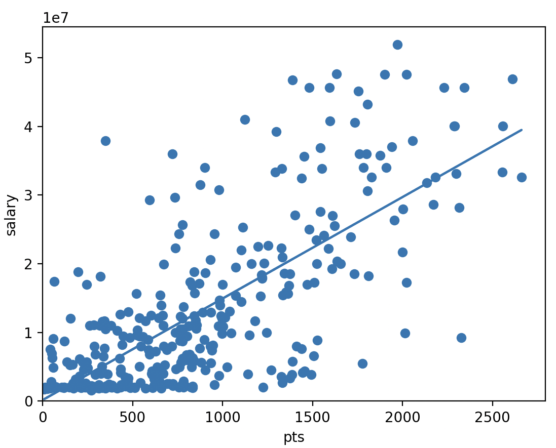
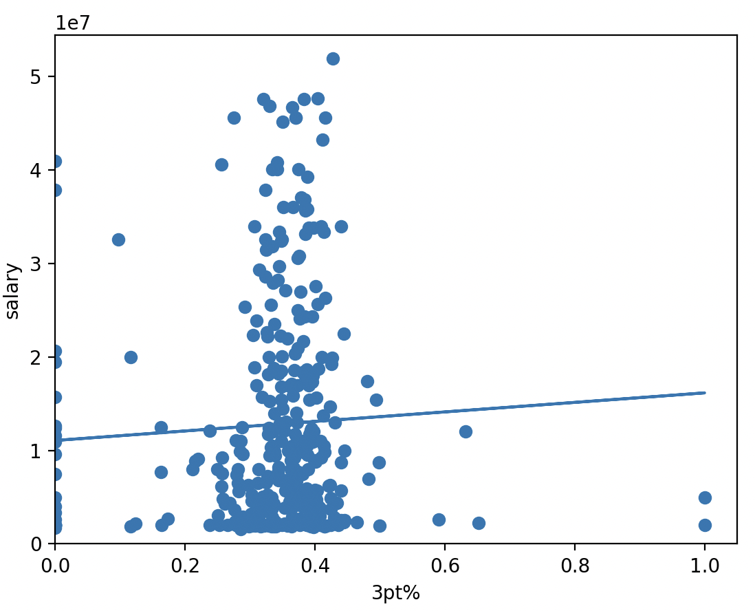
These charts show why feature selection matters. Points had a strong relationship with salary in the dataset, while three-point percentage alone was much weaker. The model works better by combining many signals instead of relying on one headline stat.
The model minimizes the gap between predicted salary and actual salary across the training data. Gradient descent repeatedly adjusts each feature weight until the cost function settles into a better fit.